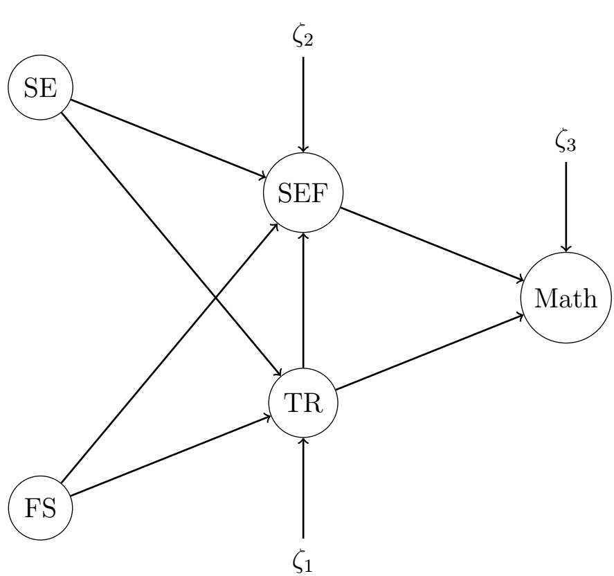
4  Application on Lavaan

Consider the following structural model:

SEM 1

where

All these variables are latent and are measured by several items.

The data are available here.

library(dplyr)

Attachement du package : 'dplyr'
Les objets suivants sont masqués depuis 'package:stats':

    filter, lag
Les objets suivants sont masqués depuis 'package:base':

    intersect, setdiff, setequal, union
library(lavaan)
This is lavaan 0.6-17
lavaan is FREE software! Please report any bugs.
library(semTools)
Warning: le package 'semTools' a été compilé avec la version R 4.3.3
 
###############################################################################
This is semTools 0.5-6
All users of R (or SEM) are invited to submit functions or ideas for functions.
###############################################################################
df<-readxl::read_xlsx("data_school.xlsx")
df%>%as_tibble()

In lavaan a latent variable is encoded by =~.

model0<-'

# measurement model 
SEF=~SEF1+SEF2+SEF3
TR=~TR1+TR2+TR3+TR4+TR5
SE=~SE1+SE2+SE3+SE4+SE5
FS=~FS1+FS2+FS3+FS4+FS5

# structural model
SEF~SE+FS
TR~SE+FS
Math~SEF+TR

'

fit0<-sem(model0,data=df)
summary(fit0)
lavaan 0.6.17 ended normally after 56 iterations

  Estimator                                         ML
  Optimization method                           NLMINB
  Number of model parameters                        44

                                                  Used       Total
  Number of observations                           291         295

Model Test User Model:
                                                      
  Test statistic                               343.650
  Degrees of freedom                               146
  P-value (Chi-square)                           0.000

Parameter Estimates:

  Standard errors                             Standard
  Information                                 Expected
  Information saturated (h1) model          Structured

Latent Variables:
                   Estimate  Std.Err  z-value  P(>|z|)
  SEF =~                                              
    SEF1              1.000                           
    SEF2              1.258    0.158    7.941    0.000
    SEF3              0.482    0.087    5.549    0.000
  TR =~                                               
    TR1               1.000                           
    TR2               0.905    0.099    9.186    0.000
    TR3               0.835    0.098    8.530    0.000
    TR4               0.705    0.087    8.145    0.000
    TR5               0.389    0.089    4.383    0.000
  SE =~                                               
    SE1               1.000                           
    SE2               1.232    0.205    6.001    0.000
    SE3               1.209    0.211    5.740    0.000
    SE4               1.395    0.235    5.949    0.000
    SE5               1.467    0.236    6.219    0.000
  FS =~                                               
    FS1               1.000                           
    FS2               0.582    0.095    6.151    0.000
    FS3               0.900    0.123    7.298    0.000
    FS4               1.092    0.144    7.586    0.000
    FS5               1.187    0.151    7.873    0.000

Regressions:
                   Estimate  Std.Err  z-value  P(>|z|)
  SEF ~                                               
    SE                1.000    0.311    3.215    0.001
    FS               -0.356    0.217   -1.639    0.101
  TR ~                                                
    SE                1.161    0.272    4.271    0.000
    FS               -0.338    0.173   -1.951    0.051
  Math ~                                              
    SEF               0.240    0.085    2.813    0.005
    TR                0.378    0.118    3.199    0.001

Covariances:
                   Estimate  Std.Err  z-value  P(>|z|)
  SE ~~                                               
    FS                0.174    0.036    4.807    0.000

Variances:
                   Estimate  Std.Err  z-value  P(>|z|)
   .SEF1              0.622    0.113    5.488    0.000
   .SEF2              0.411    0.163    2.523    0.012
   .SEF3              1.391    0.119   11.675    0.000
   .TR1               0.354    0.050    7.102    0.000
   .TR2               0.554    0.059    9.421    0.000
   .TR3               0.644    0.063   10.158    0.000
   .TR4               0.539    0.052   10.452    0.000
   .TR5               0.806    0.069   11.744    0.000
   .SE1               0.835    0.074   11.277    0.000
   .SE2               0.544    0.053   10.210    0.000
   .SE3               0.699    0.065   10.681    0.000
   .SE4               0.742    0.072   10.322    0.000
   .SE5               0.575    0.060    9.562    0.000
   .FS1               0.742    0.069   10.715    0.000
   .FS2               0.354    0.032   11.110    0.000
   .FS3               0.399    0.040   10.016    0.000
   .FS4               0.461    0.049    9.439    0.000
   .FS5               0.398    0.047    8.479    0.000
   .Math              1.396    0.118   11.806    0.000
   .SEF               0.766    0.134    5.703    0.000
   .TR                0.336    0.062    5.405    0.000
    SE                0.197    0.057    3.476    0.001
    FS                0.308    0.069    4.441    0.000

4.1 More difficult

We want to estimate the indirect effect of the two exogenous variables on math through the two mediators (TR and SEF).

It leads to estimate \[Ind_{ij}=\gamma_{ij}\times \beta_j,\] where the regressions coefficients are define from the following equations

\[ \begin{cases} TR=\gamma_{11}SE+\gamma_{21}FS, \\ SEF=\gamma_{12}SE+\gamma_{22}FS, \\ Math=\beta_1 TR+\beta_2 SEF. \end{cases} \]

See the correction
model<-'
#measurement model 
SEF=~SEF1+SEF2+SEF3
TR=~TR1+TR2+TR3+TR4+TR5
SE=~SE1+SE2+SE3+SE4+SE5
FS=~FS1+FS2+FS3+FS4+FS5

TR~g11*SE+g21*FS
SEF~g12*SE+g22*FS
Math~b1*SEF+b2*TR

I11:=g11*b1
I21:=g21*b1
I12:=g11*b2
I22:=g21*b2
'

fit<-sem(model,data=df)
summary(fit)
lavaan 0.6.17 ended normally after 56 iterations

  Estimator                                         ML
  Optimization method                           NLMINB
  Number of model parameters                        44

                                                  Used       Total
  Number of observations                           291         295

Model Test User Model:
                                                      
  Test statistic                               343.650
  Degrees of freedom                               146
  P-value (Chi-square)                           0.000

Parameter Estimates:

  Standard errors                             Standard
  Information                                 Expected
  Information saturated (h1) model          Structured

Latent Variables:
                   Estimate  Std.Err  z-value  P(>|z|)
  SEF =~                                              
    SEF1              1.000                           
    SEF2              1.258    0.158    7.941    0.000
    SEF3              0.482    0.087    5.549    0.000
  TR =~                                               
    TR1               1.000                           
    TR2               0.905    0.099    9.186    0.000
    TR3               0.835    0.098    8.530    0.000
    TR4               0.705    0.087    8.145    0.000
    TR5               0.389    0.089    4.383    0.000
  SE =~                                               
    SE1               1.000                           
    SE2               1.232    0.205    6.001    0.000
    SE3               1.209    0.211    5.740    0.000
    SE4               1.395    0.235    5.949    0.000
    SE5               1.467    0.236    6.219    0.000
  FS =~                                               
    FS1               1.000                           
    FS2               0.582    0.095    6.151    0.000
    FS3               0.900    0.123    7.298    0.000
    FS4               1.092    0.144    7.586    0.000
    FS5               1.187    0.151    7.873    0.000

Regressions:
                   Estimate  Std.Err  z-value  P(>|z|)
  TR ~                                                
    SE       (g11)    1.161    0.272    4.271    0.000
    FS       (g21)   -0.338    0.173   -1.951    0.051
  SEF ~                                               
    SE       (g12)    1.000    0.311    3.215    0.001
    FS       (g22)   -0.356    0.217   -1.639    0.101
  Math ~                                              
    SEF       (b1)    0.240    0.085    2.813    0.005
    TR        (b2)    0.378    0.118    3.199    0.001

Covariances:
                   Estimate  Std.Err  z-value  P(>|z|)
  SE ~~                                               
    FS                0.174    0.036    4.807    0.000

Variances:
                   Estimate  Std.Err  z-value  P(>|z|)
   .SEF1              0.622    0.113    5.488    0.000
   .SEF2              0.411    0.163    2.523    0.012
   .SEF3              1.391    0.119   11.675    0.000
   .TR1               0.354    0.050    7.102    0.000
   .TR2               0.554    0.059    9.421    0.000
   .TR3               0.644    0.063   10.158    0.000
   .TR4               0.539    0.052   10.452    0.000
   .TR5               0.806    0.069   11.744    0.000
   .SE1               0.835    0.074   11.277    0.000
   .SE2               0.544    0.053   10.210    0.000
   .SE3               0.699    0.065   10.681    0.000
   .SE4               0.742    0.072   10.322    0.000
   .SE5               0.575    0.060    9.562    0.000
   .FS1               0.742    0.069   10.715    0.000
   .FS2               0.354    0.032   11.110    0.000
   .FS3               0.399    0.040   10.016    0.000
   .FS4               0.461    0.049    9.439    0.000
   .FS5               0.398    0.047    8.479    0.000
   .Math              1.396    0.118   11.806    0.000
   .SEF               0.766    0.134    5.703    0.000
   .TR                0.336    0.062    5.405    0.000
    SE                0.197    0.057    3.476    0.001
    FS                0.308    0.069    4.441    0.000

Defined Parameters:
                   Estimate  Std.Err  z-value  P(>|z|)
    I11               0.279    0.118    2.367    0.018
    I21              -0.081    0.050   -1.615    0.106
    I12               0.438    0.167    2.632    0.008
    I22              -0.128    0.076   -1.686    0.092

4.2 Focus on the measurement model

In this part, we forget the structural model and we focus only on the measurement model. The first question is to check that the measures of the latent variables are consistent with the way the researcher understands those latent variables (e.g. we check that the items SEF1, SEF2, SFE3 are really associated with SEF).

model0<-'
#measurement model 
SEF=~SEF1+SEF2+SEF3
TR=~TR1+TR2+TR3+TR4+TR5
SE=~SE1+SE2+SE3+SE4+SE5
FS=~FS1+FS2+FS3+FS4+FS5
'

This is conformatory factor analysis (CFA).

fit0<-cfa(model0,data=df,meanstructure=T)

The consistency of the construction of latent variable is based on GOF indices, we must have

  • \(CFI>0.90\),

  • \(TLI>0.90\),

  • \(RMSEA < 0.08\).

fitmeasures(fit0)
                 npar                  fmin                 chisq 
               60.000                 0.417               242.418 
                   df                pvalue        baseline.chisq 
              129.000                 0.000              1416.517 
          baseline.df       baseline.pvalue                   cfi 
              153.000                 0.000                 0.910 
                  tli                  nnfi                   rfi 
                0.894                 0.894                 0.797 
                  nfi                  pnfi                   ifi 
                0.829                 0.699                 0.912 
                  rni                  logl     unrestricted.logl 
                0.910             -6747.308             -6626.099 
                  aic                   bic                ntotal 
            13614.615             13835.015               291.000 
                 bic2                 rmsea        rmsea.ci.lower 
            13644.742                 0.055                 0.044 
       rmsea.ci.upper        rmsea.ci.level          rmsea.pvalue 
                0.066                 0.900                 0.214 
       rmsea.close.h0 rmsea.notclose.pvalue     rmsea.notclose.h0 
                0.050                 0.000                 0.080 
                  rmr            rmr_nomean                  srmr 
                0.071                 0.075                 0.069 
         srmr_bentler   srmr_bentler_nomean                  crmr 
                0.069                 0.073                 0.073 
          crmr_nomean            srmr_mplus     srmr_mplus_nomean 
                0.077                 0.069                 0.073 
                cn_05                 cn_01                   gfi 
              188.873               204.203                 0.989 
                 agfi                  pgfi                   mfi 
                0.984                 0.675                 0.823 
                 ecvi 
                1.245 

4.3 Invariance of the measurement model

All the issues of this section are extracted from .

Let’s look at the question of the difference in self-efficacy feeling between boys and girls. The most common way to do this is to compare group means by a Student test. But, this requires that

  • boys and girls understand and react similarly to the questions,

  • the response models should be invariant across gender.

To assess these assumptions, the measurement models are tested against an increasing number of constraints. All these models are nested.

Fisrt step: Configural model. The invariance of the model form is checked: do the latent variables follow the same pattern across genders? (i.e. same items are associated with same latent variables for boys and girls).

fit_config<-cfa(model0,data=df,group="gender",meanstructure=T)
fitmeasures(fit_config)
                 npar                  fmin                 chisq 
              120.000                 0.665               387.086 
                   df                pvalue        baseline.chisq 
              258.000                 0.000              1492.165 
          baseline.df       baseline.pvalue                   cfi 
              306.000                 0.000                 0.891 
                  tli                  nnfi                   rfi 
                0.871                 0.871                 0.692 
                  nfi                  pnfi                   ifi 
                0.741                 0.624                 0.895 
                  rni                  logl     unrestricted.logl 
                0.891             -6660.526             -6466.983 
                  aic                   bic                ntotal 
            13561.051             14001.850               291.000 
                 bic2                 rmsea        rmsea.ci.lower 
            13621.305                 0.059                 0.046 
       rmsea.ci.upper        rmsea.ci.level          rmsea.pvalue 
                0.070                 0.900                 0.121 
       rmsea.close.h0 rmsea.notclose.pvalue     rmsea.notclose.h0 
                0.050                 0.001                 0.080 
                  rmr            rmr_nomean                  srmr 
                0.081                 0.085                 0.081 
         srmr_bentler   srmr_bentler_nomean                  crmr 
                0.081                 0.085                 0.085 
          crmr_nomean            srmr_mplus     srmr_mplus_nomean 
                0.090                 0.081                 0.085 
                cn_05                 cn_01                   gfi 
              223.875               236.880                 0.986 
                 agfi                  pgfi                   mfi 
                0.980                 0.673                 0.801 
                 ecvi 
                2.155 

According to the criteria defined above for the GOF indices, this model is acceptable. However, it is necessary to check that it fits the data as well as the model without gender. As these two models are nested, the difference between them can be assessed on the basis of the significance of the change in \(\chi^2.\).

lavTestLRT(fit0,fit_config)

However, as usually this test is sensible to the sample size, thus alternative fit indices comparisons are used in application. The differences in CFI (\(\Delta CFI\)) and RMSEA (\(\Delta RMSEA\)) are the most commonly used and may not exceed 0.01 in absolute value.

fitmeasures(fit_config)["cfi"]-fitmeasures(fit0)["cfi"]
        cfi 
-0.01906258 
fitmeasures(fit_config)["rmsea"]-fitmeasures(fit0)["rmsea"]
      rmsea 
0.003673898 

4.3.1 Constraints on measurement model parameters

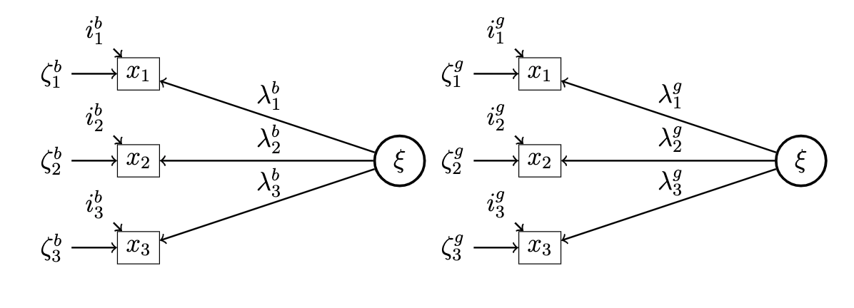
For all the latent of the configural model, the following diagram describes the measurement model:

configural invariance Second step: Weak invariance (or metric invariance). If weak invariance is supported, the equivalence of the item loadings on the latent variable is tested. Metric invariance means that each item contributes to the latent construct to a similar degree across groups. With previous notations the null hypothesis is \[ \begin{cases} \lambda^g_1=\lambda^b_1, \\ \lambda^g_2=\lambda^b_2, \\ \dots \end{cases} \]

fit_weak<-cfa(model0,data=df,group="gender",group.equal="loadings")
lavTestLRT(fit_config,fit_weak)
fitmeasures(fit_config)["cfi"]-fitmeasures(fit_weak)["cfi"]
        cfi 
0.004197831 
fitmeasures(fit_config)["rmsea"]-fitmeasures(fit_weak)["rmsea"]
      rmsea 
0.000437986 

Third step: Strong invariance (or scalar invariance). If weak invariance is supported, the equivalence of the item intercept on the latent variable is tested. Scalar invariance means that mean differences in the latent construct capture all mean differences in the shared variance of the items. With previous notations the null hypothesis is

\[ \begin{cases} i^g_1=i^b_1, \\ i^g_2=i^b_2, \\ \dots \end{cases} \]

fit_strong<-cfa(model0,data=df,group="gender",group.equal=c("loadings","intercepts"))
lavTestLRT(fit_weak,fit_strong)
fitmeasures(fit_strong)["cfi"]-fitmeasures(fit_weak)["cfi"]
        cfi 
-0.01402527 
fitmeasures(fit_strong)["rmsea"]-fitmeasures(fit_weak)["rmsea"]
      rmsea 
0.001976347 

Strong invariance cannot be supported. To improve the fit of the model, we can assume that strong invariance is true, with the exception of some items that need to be identified.

parameterestimates(fit_weak)%>%filter(op=="~1"&group=="1"&est!=0)
parameterestimates(fit_weak)%>%filter(op=="~1"&group=="2"&est!=0)

Let consider the difference in intercept estimations :

tab1<-parameterestimates(fit_weak)%>%filter(op=="~1"&group=="1"&est!=0)
tab2<-parameterestimates(fit_weak)%>%filter(op=="~1"&group=="2"&est!=0)
diff<-tab1[,"est"]-tab2[,"est"]
names(diff)<-tab1$lhs
diff
      SEF1       SEF2       SEF3        TR1        TR2        TR3        TR4 
0.02743321 0.37953244 0.37003817 0.21879771 0.13573473 0.26216603 0.11894084 
       TR5        SE1        SE2        SE3        SE4        SE5        FS1 
0.14751908 0.50725191 0.13382634 0.53392176 0.44518130 0.38645038 0.44160305 
       FS2        FS3        FS4        FS5 
0.30152672 0.27733779 0.42461832 0.48296756 

Removing the equality constraint on items can be achieved using group.partial

fit_strong2<-cfa(model0,data=df,group="gender",group.equal=c("loadings","intercepts"),group.partial="SE4~1")
lavTestLRT(fit_weak,fit_strong2)
fitmeasures(fit_strong2)["cfi"]-fitmeasures(fit_weak)["cfi"]
        cfi 
-0.01478964 
fitmeasures(fit_strong2)["rmsea"]-fitmeasures(fit_weak)["rmsea"]
      rmsea 
0.002262904 
fit_strong3<-cfa(model0,data=df,group="gender",group.equal=c("loadings","intercepts"),group.partial=c("SE2~1","SE4~1"))
lavTestLRT(fit_weak,fit_strong3)
fitmeasures(fit_strong3)["cfi"]-fitmeasures(fit_weak)["cfi"]
         cfi 
-0.009050069 
fitmeasures(fit_strong3)["rmsea"]-fitmeasures(fit_weak)["rmsea"]
       rmsea 
0.0009936305 

4.4 Moderation modelling

In this section we look for gender invariance in the mediation model examined above. More specifically, is this mediation model the same for male and female students?

model0<-'
# measurement model 
SEF=~SEF1+SEF2+SEF3
TR=~TR1+TR2+TR3+TR4+TR5
SE=~SE1+SE2+SE3+SE4+SE5
FS=~FS1+FS2+FS3+FS4+FS5

# structural model
SEF~SE+FS
TR~SE+FS
Math~SEF+TR

# constraint
TR~~0*TR
'

fit0<-sem(model0,data=df,group="gender",group.equal=c("loadings","intercepts","regressions"),group.partial=c("SE2~1","SE4~1"))

fit1<-sem(model0,data=df,group="gender",group.equal=c("loadings","intercepts"),group.partial=c("SE2~1","SE4~1"))

lavTestLRT(fit0,fit1)