2  Example in Lavaan

Download the following data_PM and open it into R.

2.1 First model

df<-readxl::read_excel("data_PM.xlsx") 
library(lavaan)

This is lavaan 0.6-17
lavaan is FREE software! Please report any bugs.

model<-"
Y1~X1
Y2~Y1+X1
"

fit1<-sem(model,data=df)

summary(fit1)

lavaan 0.6.17 ended normally after 1 iteration

  Estimator                                         ML
  Optimization method                           NLMINB
  Number of model parameters                         5

  Number of observations                           100

Model Test User Model:
                                                      
  Test statistic                                 0.000
  Degrees of freedom                                 0

Parameter Estimates:

  Standard errors                             Standard
  Information                                 Expected
  Information saturated (h1) model          Structured

Regressions:
                   Estimate  Std.Err  z-value  P(>|z|)
  Y1 ~                                                
    X1                1.004    0.048   20.880    0.000
  Y2 ~                                                
    Y1                2.018    0.210    9.592    0.000
    X1                1.001    0.234    4.273    0.000

Variances:
                   Estimate  Std.Err  z-value  P(>|z|)
   .Y1                0.985    0.139    7.071    0.000
   .Y2                4.360    0.617    7.071    0.000

We can compare the empirical covariance matrix:

n<-dim(df)[1]
round(cov(df)*(n-1)/n,3)

       Y1     Y2     X1
Y1  5.280 14.935  4.276
Y2 14.935 47.405 12.891
X1  4.276 12.891  4.258

to the fitted covariance matrix

fitted(fit1)

$cov
       Y1     Y2     X1
Y1  5.280              
Y2 14.935 47.405       
X1  4.276 12.891  4.258

2.1.1 Remarks:

• The degree of freedom of the model is 0 (6 parameters to be estimated from 6 observed values).

• We can perform two OLS regression and we will find the same solutions.

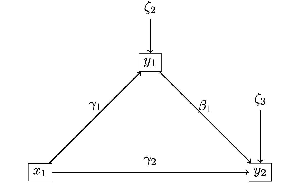
One of the avantage of the Path-modelling is to test the existence of the indirect effect \(I=\gamma_1\beta_1\) of \(\xi_1\) on \(\eta_2\). In the following code, we define this inidrect effect through the symbol :=

model<-"
Y1~g1*X1
Y2~b1*Y1+g2*X1
I:=g1*b1
"

fit1<-sem(model,data=df)
summary(fit1)

lavaan 0.6.17 ended normally after 1 iteration

  Estimator                                         ML
  Optimization method                           NLMINB
  Number of model parameters                         5

  Number of observations                           100

Model Test User Model:
                                                      
  Test statistic                                 0.000
  Degrees of freedom                                 0

Parameter Estimates:

  Standard errors                             Standard
  Information                                 Expected
  Information saturated (h1) model          Structured

Regressions:
                   Estimate  Std.Err  z-value  P(>|z|)
  Y1 ~                                                
    X1        (g1)    1.004    0.048   20.880    0.000
  Y2 ~                                                
    Y1        (b1)    2.018    0.210    9.592    0.000
    X1        (g2)    1.001    0.234    4.273    0.000

Variances:
                   Estimate  Std.Err  z-value  P(>|z|)
   .Y1                0.985    0.139    7.071    0.000
   .Y2                4.360    0.617    7.071    0.000

Defined Parameters:
                   Estimate  Std.Err  z-value  P(>|z|)
    I                 2.027    0.233    8.716    0.000

2.2 Second model

Build on lavaan the model corresponding to this path diagram:

See the correction

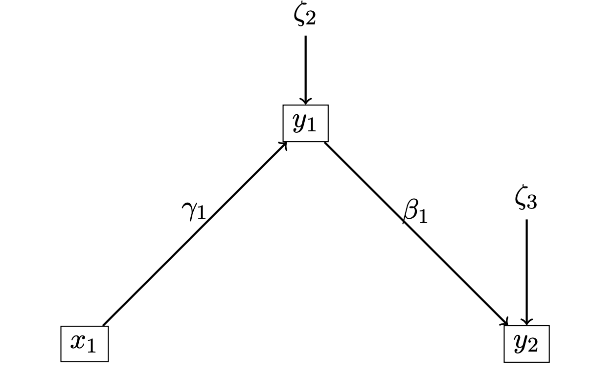
model<-"
Y1~a*X1
Y2~b*Y1
I:=a*b
"

fit1<-sem(model,data=df)
summary(fit1)

lavaan 0.6.17 ended normally after 1 iteration

  Estimator                                         ML
  Optimization method                           NLMINB
  Number of model parameters                         4

  Number of observations                           100

Model Test User Model:
                                                      
  Test statistic                                16.767
  Degrees of freedom                                 1
  P-value (Chi-square)                           0.000

Parameter Estimates:

  Standard errors                             Standard
  Information                                 Expected
  Information saturated (h1) model          Structured

Regressions:
                   Estimate  Std.Err  z-value  P(>|z|)
  Y1 ~                                                
    X1         (a)    1.004    0.048   20.880    0.000
  Y2 ~                                                
    Y1         (b)    2.829    0.099   28.625    0.000

Variances:
                   Estimate  Std.Err  z-value  P(>|z|)
   .Y1                0.985    0.139    7.071    0.000
   .Y2                5.156    0.729    7.071    0.000

Defined Parameters:
                   Estimate  Std.Err  z-value  P(>|z|)
    I                 2.841    0.168   16.869    0.000