3 Covariance analysis for SEM
3.1 Latent variables
Latent variables (or hidden variables) play a central role in a wide range of scientific fields, including psychology, medicine and economics.
These variables can not directly observed and can be inferred only indirectly from observable variables.
Example: Intelligence of Children calculated from the fith WISC (Wechsler Intelligence Scale for Children)
3.2 Structure of a SEM
Structural model: linear relationship between latent variables.
Measurement model: linear relationship between a latent variable and its indicators.
3.3 Example of SEM:
This study was carried out in the Nantes area in 2017.
The main issue of this study: Which psychological variables predict academic performances in mathematics and french?
Three latent variables are involved in the model:
relationship with the teacher,
self-efficacy feeling,
academic performance in mathematics.
3.4 Diagram of the model:
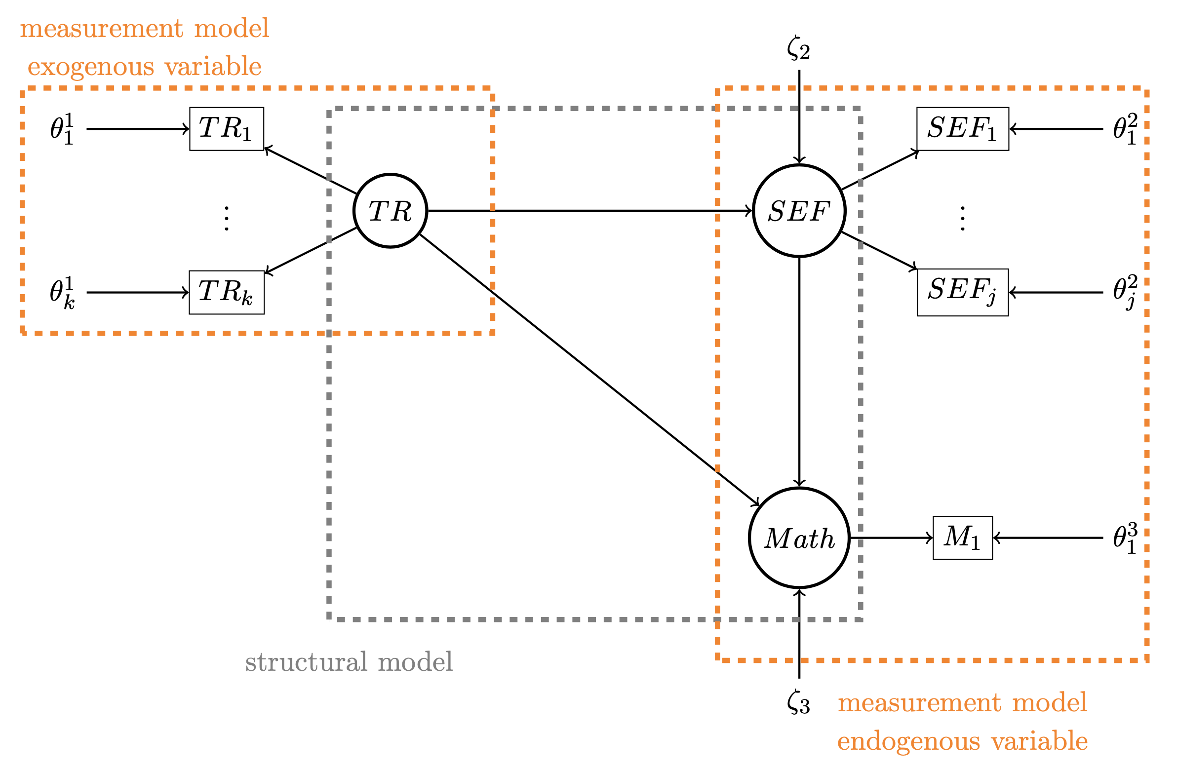
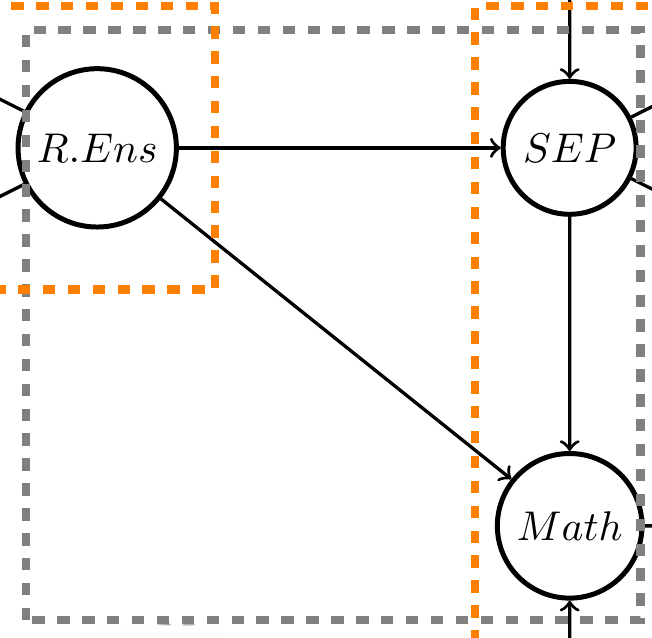
3.5 Structural model (gray)
A good relationship with the teacher (R.Ens) increases the self efficacy feeling (SEP) which, its turn, leads to better performances in mathematics.
\[ \begin{cases} \eta_1=\gamma_1 \xi_1 +\zeta_1 \\ \eta_2=\beta_1 \eta_1 + \gamma_2\xi_1 +\zeta_2 \end{cases} \] where \(\eta_\bullet\) denotes the endogenous variables and \(\xi_\bullet\) the exogenous variables.
\(\eta_1:\) self efficacy feeling, \(\eta_2:\) math performance, \(\xi_1:\) relationship with the teacher.
3.6 Measurement model
Three latent variables are involved in the model:
relationship with the teacher: five items were proposed to the children.
self-efficacy feeling:
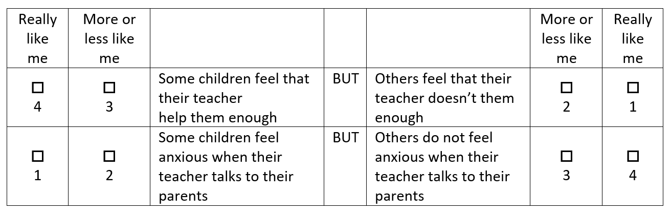
3.7 Example of items for the relationship with the teacher
I’m going to ask you some questions about yourself and about school. I want to know what you’re like when you’re at school. Let me explain these questions first. Each question is about two types of child and I want to know which one is more like you.
3.8 Reflective model
In this model, we assume that latent variable predicts item covariances:
Example: \(\xi_1\) relationship with teacher measured by 5 items \(x_1,...,x_5\) on a Likert scale (i.e. level of agreement or disagreement with a statement) from 1 to 4 .
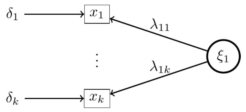
Observable variables are written as:
\[ x_i=\lambda_{1i}\xi_1+\delta_i \]
3.9 Usual notations in covariance analysis
Let \(x_1,...,x_p\) the observable variables corresponding to an exogenous latent variable \(\xi\) and \(y_1,...,y_p\) the observable variables of an endogenous latent variable \(\eta\).
- Measurement model: \[ \bf{y}=\Lambda_y \eta +\varepsilon, \quad \bf{x}=\Lambda_x \xi +\delta. \]
- Structural model:
\[\eta=\bf{B}\eta+\Gamma\xi+\zeta.\]
3.10 Assumptions
The assumptions on the latent variables are the same as those on the observed variables for path modelling.
3.11 GOF indices in SEM
The most popular are CFI, TLI and RMSEA.
The relative GOF are often used to evaluate the measurement model while the absolute GOF evaluate the structural model.