1 Covariance Analysis for Path model
The path analysis concerns observed variables only. In this case, the exogenous variables are denoted by \(x_\bullet\) and the endogenous variables are denoted by \(y_\bullet.\)
1.1 Limits of regression model
Regression models are popular for testing linear relationship between continous predictors and continous outcome.
However, in this framework :
- Predictors are measured without errors.
- For example, some systems of regression equations cannot be tested:
1.2 Assumptions
We assume that the errors \(\zeta_\bullet\) are not correlated.
Moreover, by definition of exogenous variables,
the errors \(\zeta_\bullet\) and the exogenous variables \(x_\bullet\) of the model are not correlated.
For simplification, we assume that endogenous and exogenous variables are standardized, that is
\[\mathbb{E}(x_\bullet)=\mathbb{E}(y_\bullet)=0, \quad \mathbb{V}(x_\bullet)=\mathbb{V}(y_\bullet)=1.\]
1.2.1 Remark :
This assumption is not necessary in the applications; it only serves to simplify the mathematical expression of the covariance matrix.
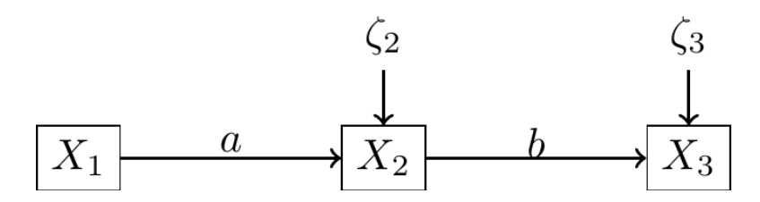
1.3 Diagram of a path
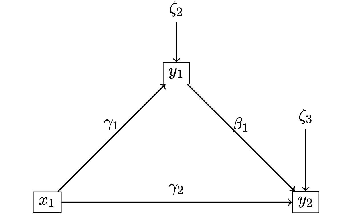
A path model can be summarized by a diagram. In the left, the diagram describes a mediation model with an exogenous variable \(x_1\), a mediator \(y_1\) and an outcome \(y_2\).
This diagram represents the following system
\[ \begin{cases} y_1=\gamma_1 x_1 +\zeta_1 \\ y_2=\beta_1 y_1 + \gamma_2x_1 +\zeta_2 \end{cases} \]
1.4 Parameters of the model
In path modelling, we assume that the \(\zeta_\bullet\) errors are centered (ie zero mean) and we denote their variances by \(\sigma^2_\bullet.\)
Let \(\theta=(\gamma_1,\beta_1,\gamma_2,\sigma_1,\sigma_2)\) the vector of parameters.
We can write the correlation matrix of the model \[ \Sigma(\theta)=\left( \begin{array}{ccc} 1 & \gamma1 & \gamma_1\beta_1+\gamma_2 \\ & \gamma_1^2+\sigma_1^2 & \beta_1+\gamma_1\gamma_2 \\ & & \gamma_2^2+\beta_1^2+\beta_1\gamma_1\gamma_2+\sigma_2^2 \end{array} \right) \]
1.5 Covariance analysis
We denote by \(S\) the empirical correlation matrix. We look for the parameter \(\theta\) such as
\[ \Sigma(\theta) \simeq S \] For Ordinary Least Square minimization, the cost function is
\[F_{ULS}=\frac1{2}\Vert \Sigma-S\Vert^2=trace[(\Sigma-S)^T.(\Sigma-S)].\]
Numerical algoritm can be performed to estimate the solution of this problem.
1.6 General problem of identification
\(q\) exogenous variables \(x_1,...,x_q\)
\(p\) endogenous variables \(y_1,...,y_p\).
\(\theta\) vector of \(t\) parameters to be estimated.
We must have:
\[ t\leq\frac{(p+q)(p+q+1)}{2} \]
1.7 Jöreskog formula
This formula provided an explicit form of the covariance matrix \(\Sigma(\theta)\) from the parameters \(\theta\) of the Path-model.
1.8 Maximum likelihood estimation
\((x_1,...,x_p,y_1,...,y_q)^T \sim \mathcal N (0,\Sigma)\), where \(\Sigma\) is the covariance matrix of the variable \(\bf{x,y}\).
\(\Sigma\) and \(S\) are positive-definite.
We define the log-likelihood function of the path model
\[F_{ML}(\theta)=\log|\Sigma|+trace(S\Sigma^{-1})-\log|S|-(p+q).\]
1.9 Properties
1.10 The cost function \(F_{ML}\)
\(F_{ML}(S,\Sigma(\theta))\geq 0,\)
\(F_{ML}(S,\Sigma(\theta))= 0\) if and only if \(S= \Sigma(\theta)),\)
\(F_{ML}\) is continuous in \(S\) as well as in \(Sigma(\theta).\)
1.11 The ML-estimator
The maximum of the function \(F_{ML}\) has no explicit expression, but it can be numerically estimated (see Jöreskog (1966)).
Asymptotically, \(\widehat \theta_{ML}\) is unbiased, consistent, efficient (i.e. among the consistent estimators of \(\theta\) it has the smallest asymptotic variance).
\(\leadsto\) Tests can be built using the previous property.
1.12 Chi-Square Test of Model Fit
It tests the null hypothesis \[H_0:\Sigma(\theta)=\Sigma.\] (i.e. implied covariance matrix equal to population covariance matrix) Under \(H_0\), its statistical is distributed from a chi-square with \(df=\frac{(p+q)(p+q+1)}{2}-t.\)
Drawback of the test: it tends to be highly powered with large samples i.e. null hypothesis is always rejected ….
\(\leadsto\) goodness of fit indices (GOF) have been introduced since 50 years.
Relative GOF compare the implied model to a baseline model which assumes all the variables have variance but no covariance (for instance CFI,TLI).
Absolute GOF (for instance RMSEA).