Le diaporama :
Test de student sur groupes indépendants
Loading required package: survival
data ("neuropathy" )library (BayesFactor)
Loading required package: coda
Loading required package: Matrix
************
Welcome to BayesFactor 0.9.12-4.7. If you have questions, please contact Richard Morey (richarddmorey@gmail.com).

Type BFManual() to open the manual.
************
library (ggplot2)library (dplyr)
Attaching package: 'dplyr'
The following object is masked from 'package:kableExtra':

    group_rows
The following objects are masked from 'package:stats':

    filter, lag
The following objects are masked from 'package:base':

    intersect, setdiff, setequal, union
= neuropathy |> filter (group== "control" ) |> select (pain) |> unlist ()= neuropathy |> filter (group== "treat" ) |> select (pain) |> unlist ()ttestBF (x,y,rscale= 1 )
Bayes factor analysis
--------------
[1] Alt., r=1 : 0.4360155 ±0.02%

Against denominator:
  Null, mu1-mu2 = 0
---
Bayes factor type: BFindepSample, JZS
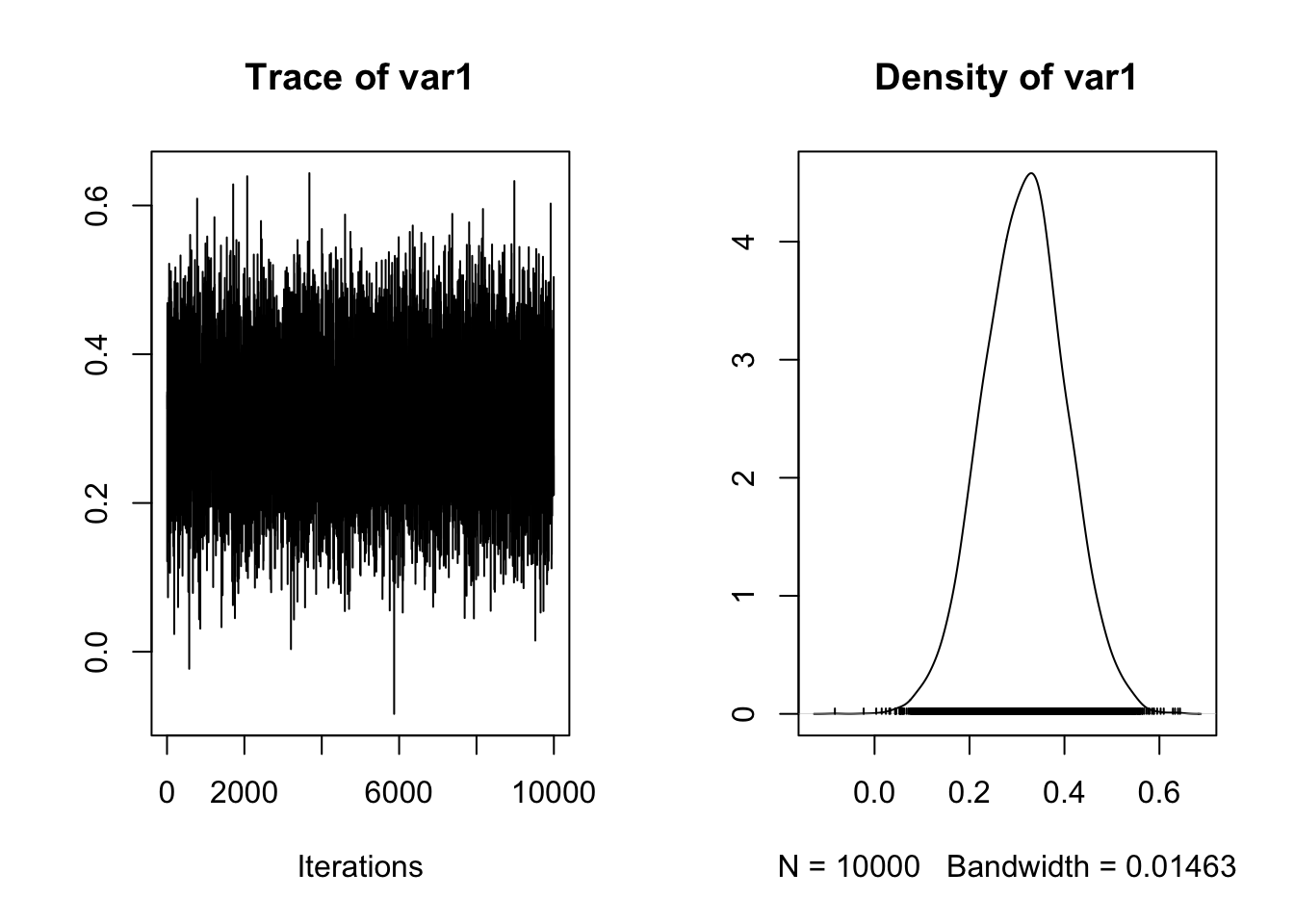
# La loi a posteriori de la différence des moyennes = ttestBF (x,y,posterior = TRUE , iterations = 10000 )plot (samples[,"mu" ])
Un autre exemple :
On s’interesse aux trois questions suivantes :
Le taux de mercure présent dans le sang est-il significativement supérieur chez le groupe exposé ?
La proportion de cellules avec des anomalies structurales est-elle significativement supérieure chez le groupe exposé ?
Test de student sur groupes appariés
L’argument paired=T permet de faire des tests sur groupes appariés :
library (carData)data ("OBrienKaiserLong" )= OBrienKaiserLong |> filter (phase %in% c ("pre" ,"post" )) |> select (score,phase)
Faire le test Bayésien de Student :
Show the code
= data |> filter (phase== "pre" ) |> select (score) |> unlist ()= data |> filter (phase== "post" ) |> select (score) |> unlist ()ttestBF (x,y,paired= T,rscale= 1 )
Bayes factor analysis
--------------
[1] Alt., r=1 : 81325.58 ±0%

Against denominator:
  Null, mu = 0
---
Bayes factor type: BFoneSample, JZS
Show the code
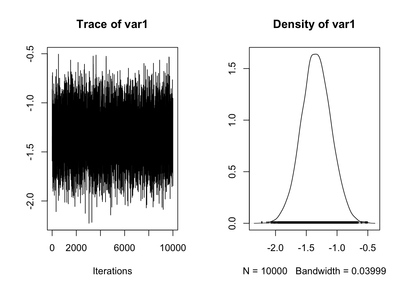
# La loi a posteriori de la différence des moyennes = ttestBF (x,y,paired= T,posterior = TRUE , iterations = 10000 )plot (samples[,"mu" ])
Régression linéaire Bayésienne
Pour calculer les facteurs de Bayes :
data ("attitude" )= regressionBF (rating ~ ., data = attitude, progress= TRUE )
  |
  |                                                                      |   0%
  |
  |=                                                                     |   2%
  |
  |==                                                                    |   3%
  |
  |===                                                                   |   5%
  |
  |====                                                                  |   6%
  |
  |======                                                                |   8%
  |
  |=======                                                               |  10%
  |
  |========                                                              |  11%
  |
  |=========                                                             |  13%
  |
  |==========                                                            |  14%
  |
  |===========                                                           |  16%
  |
  |============                                                          |  17%
  |
  |=============                                                         |  19%
  |
  |==============                                                        |  21%
  |
  |================                                                      |  22%
  |
  |=================                                                     |  24%
  |
  |==================                                                    |  25%
  |
  |===================                                                   |  27%
  |
  |====================                                                  |  29%
  |
  |=====================                                                 |  30%
  |
  |======================                                                |  32%
  |
  |=======================                                               |  33%
  |
  |========================                                              |  35%
  |
  |==========================                                            |  37%
  |
  |===========================                                           |  38%
  |
  |============================                                          |  40%
  |
  |=============================                                         |  41%
  |
  |==============================                                        |  43%
  |
  |===============================                                       |  44%
  |
  |================================                                      |  46%
  |
  |=================================                                     |  48%
  |
  |==================================                                    |  49%
  |
  |====================================                                  |  51%
  |
  |=====================================                                 |  52%
  |
  |======================================                                |  54%
  |
  |=======================================                               |  56%
  |
  |========================================                              |  57%
  |
  |=========================================                             |  59%
  |
  |==========================================                            |  60%
  |
  |===========================================                           |  62%
  |
  |============================================                          |  63%
  |
  |==============================================                        |  65%
  |
  |===============================================                       |  67%
  |
  |================================================                      |  68%
  |
  |=================================================                     |  70%
  |
  |==================================================                    |  71%
  |
  |===================================================                   |  73%
  |
  |====================================================                  |  75%
  |
  |=====================================================                 |  76%
  |
  |======================================================                |  78%
  |
  |========================================================              |  79%
  |
  |=========================================================             |  81%
  |
  |==========================================================            |  83%
  |
  |===========================================================           |  84%
  |
  |============================================================          |  86%
  |
  |=============================================================         |  87%
  |
  |==============================================================        |  89%
  |
  |===============================================================       |  90%
  |
  |================================================================      |  92%
  |
  |==================================================================    |  94%
  |
  |===================================================================   |  95%
  |
  |====================================================================  |  97%
  |
  |===================================================================== |  98%
  |
  |======================================================================| 100%
Bayes factor analysis
--------------
[1] complaints                      : 417938.6 ±0.01%
[2] complaints + learning           : 207271.9 ±0%
[3] complaints + learning + advance : 88041.54 ±0%
[4] complaints + raises             : 77498.99 ±0%
[5] complaints + privileges         : 75015.23 ±0%
[6] complaints + advance            : 72759.76 ±0%

Against denominator:
  Intercept only
---
Bayes factor type: BFlinearModel, JZS
head (res/ res[length (res)])
Bayes factor analysis
--------------
[1] complaints                      : 188.949  ±0.01%
[2] complaints + learning           : 93.70711 ±0%
[3] complaints + learning + advance : 39.80336 ±0%
[4] complaints + raises             : 35.0371  ±0%
[5] complaints + privileges         : 33.9142  ±0%
[6] complaints + advance            : 32.89451 ±0%

Against denominator:
  rating ~ complaints + privileges + learning + raises + critical + advance
---
Bayes factor type: BFlinearModel, JZS
Pour calculer les coefficients du modèle :
Loading required package: Rcpp
This is rstanarm version 2.32.1
- See https://mc-stan.org/rstanarm/articles/priors for changes to default priors!
- Default priors may change, so it's safest to specify priors, even if equivalent to the defaults.
- For execution on a local, multicore CPU with excess RAM we recommend calling
options(mc.cores = parallel::detectCores())
<- stan_glm (rating ~ ., data = attitude, seed= 44 )
SAMPLING FOR MODEL 'continuous' NOW (CHAIN 1).
Chain 1:
Chain 1: Gradient evaluation took 0.000653 seconds
Chain 1: 1000 transitions using 10 leapfrog steps per transition would take 6.53 seconds.
Chain 1: Adjust your expectations accordingly!
Chain 1:
Chain 1:
Chain 1: Iteration:    1 / 2000 [  0%]  (Warmup)
Chain 1: Iteration:  200 / 2000 [ 10%]  (Warmup)
Chain 1: Iteration:  400 / 2000 [ 20%]  (Warmup)
Chain 1: Iteration:  600 / 2000 [ 30%]  (Warmup)
Chain 1: Iteration:  800 / 2000 [ 40%]  (Warmup)
Chain 1: Iteration: 1000 / 2000 [ 50%]  (Warmup)
Chain 1: Iteration: 1001 / 2000 [ 50%]  (Sampling)
Chain 1: Iteration: 1200 / 2000 [ 60%]  (Sampling)
Chain 1: Iteration: 1400 / 2000 [ 70%]  (Sampling)
Chain 1: Iteration: 1600 / 2000 [ 80%]  (Sampling)
Chain 1: Iteration: 1800 / 2000 [ 90%]  (Sampling)
Chain 1: Iteration: 2000 / 2000 [100%]  (Sampling)
Chain 1:
Chain 1:  Elapsed Time: 0.059 seconds (Warm-up)
Chain 1:                0.051 seconds (Sampling)
Chain 1:                0.11 seconds (Total)
Chain 1:

SAMPLING FOR MODEL 'continuous' NOW (CHAIN 2).
Chain 2:
Chain 2: Gradient evaluation took 2.7e-05 seconds
Chain 2: 1000 transitions using 10 leapfrog steps per transition would take 0.27 seconds.
Chain 2: Adjust your expectations accordingly!
Chain 2:
Chain 2:
Chain 2: Iteration:    1 / 2000 [  0%]  (Warmup)
Chain 2: Iteration:  200 / 2000 [ 10%]  (Warmup)
Chain 2: Iteration:  400 / 2000 [ 20%]  (Warmup)
Chain 2: Iteration:  600 / 2000 [ 30%]  (Warmup)
Chain 2: Iteration:  800 / 2000 [ 40%]  (Warmup)
Chain 2: Iteration: 1000 / 2000 [ 50%]  (Warmup)
Chain 2: Iteration: 1001 / 2000 [ 50%]  (Sampling)
Chain 2: Iteration: 1200 / 2000 [ 60%]  (Sampling)
Chain 2: Iteration: 1400 / 2000 [ 70%]  (Sampling)
Chain 2: Iteration: 1600 / 2000 [ 80%]  (Sampling)
Chain 2: Iteration: 1800 / 2000 [ 90%]  (Sampling)
Chain 2: Iteration: 2000 / 2000 [100%]  (Sampling)
Chain 2:
Chain 2:  Elapsed Time: 0.065 seconds (Warm-up)
Chain 2:                0.043 seconds (Sampling)
Chain 2:                0.108 seconds (Total)
Chain 2:

SAMPLING FOR MODEL 'continuous' NOW (CHAIN 3).
Chain 3:
Chain 3: Gradient evaluation took 6e-06 seconds
Chain 3: 1000 transitions using 10 leapfrog steps per transition would take 0.06 seconds.
Chain 3: Adjust your expectations accordingly!
Chain 3:
Chain 3:
Chain 3: Iteration:    1 / 2000 [  0%]  (Warmup)
Chain 3: Iteration:  200 / 2000 [ 10%]  (Warmup)
Chain 3: Iteration:  400 / 2000 [ 20%]  (Warmup)
Chain 3: Iteration:  600 / 2000 [ 30%]  (Warmup)
Chain 3: Iteration:  800 / 2000 [ 40%]  (Warmup)
Chain 3: Iteration: 1000 / 2000 [ 50%]  (Warmup)
Chain 3: Iteration: 1001 / 2000 [ 50%]  (Sampling)
Chain 3: Iteration: 1200 / 2000 [ 60%]  (Sampling)
Chain 3: Iteration: 1400 / 2000 [ 70%]  (Sampling)
Chain 3: Iteration: 1600 / 2000 [ 80%]  (Sampling)
Chain 3: Iteration: 1800 / 2000 [ 90%]  (Sampling)
Chain 3: Iteration: 2000 / 2000 [100%]  (Sampling)
Chain 3:
Chain 3:  Elapsed Time: 0.063 seconds (Warm-up)
Chain 3:                0.052 seconds (Sampling)
Chain 3:                0.115 seconds (Total)
Chain 3:

SAMPLING FOR MODEL 'continuous' NOW (CHAIN 4).
Chain 4:
Chain 4: Gradient evaluation took 8e-06 seconds
Chain 4: 1000 transitions using 10 leapfrog steps per transition would take 0.08 seconds.
Chain 4: Adjust your expectations accordingly!
Chain 4:
Chain 4:
Chain 4: Iteration:    1 / 2000 [  0%]  (Warmup)
Chain 4: Iteration:  200 / 2000 [ 10%]  (Warmup)
Chain 4: Iteration:  400 / 2000 [ 20%]  (Warmup)
Chain 4: Iteration:  600 / 2000 [ 30%]  (Warmup)
Chain 4: Iteration:  800 / 2000 [ 40%]  (Warmup)
Chain 4: Iteration: 1000 / 2000 [ 50%]  (Warmup)
Chain 4: Iteration: 1001 / 2000 [ 50%]  (Sampling)
Chain 4: Iteration: 1200 / 2000 [ 60%]  (Sampling)
Chain 4: Iteration: 1400 / 2000 [ 70%]  (Sampling)
Chain 4: Iteration: 1600 / 2000 [ 80%]  (Sampling)
Chain 4: Iteration: 1800 / 2000 [ 90%]  (Sampling)
Chain 4: Iteration: 2000 / 2000 [100%]  (Sampling)
Chain 4:
Chain 4:  Elapsed Time: 0.075 seconds (Warm-up)
Chain 4:                0.049 seconds (Sampling)
Chain 4:                0.124 seconds (Total)
Chain 4:
print (model_bayes, digits = 3 )
stan_glm
 family:       gaussian [identity]
 formula:      rating ~ .
 observations: 30
 predictors:   7
------
            Median MAD_SD
(Intercept) 11.029 11.762
complaints   0.615  0.164
privileges  -0.069  0.140
learning     0.312  0.173
raises       0.082  0.224
critical     0.037  0.151
advance     -0.216  0.185

Auxiliary parameter(s):
      Median MAD_SD
sigma 7.231  1.106

------
* For help interpreting the printed output see ?print.stanreg
* For info on the priors used see ?prior_summary.stanreg
This is bayesplot version 1.11.1
- Online documentation and vignettes at mc-stan.org/bayesplot
- bayesplot theme set to bayesplot::theme_default()
* Does _not_ affect other ggplot2 plots
* See ?bayesplot_theme_set for details on theme setting
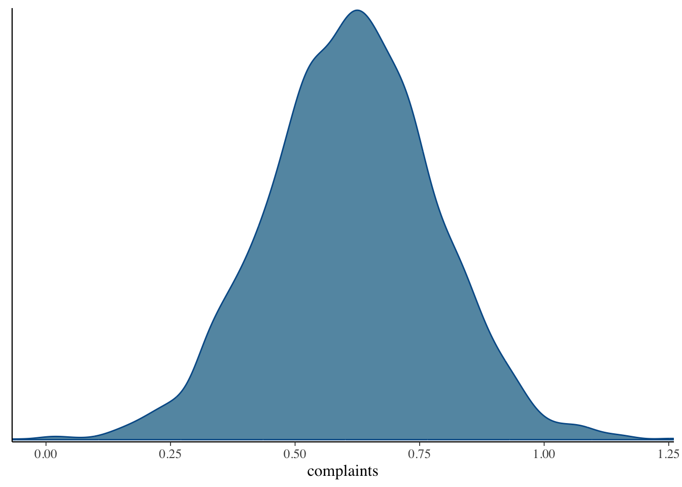
mcmc_dens (model_bayes, pars = c ("complaints" ))library (bayestestR)hdi (model_bayes)
Highest Density Interval

Parameter   |         95% HDI
-----------------------------
(Intercept) | [-13.50, 34.39]
complaints  | [  0.30,  0.95]
privileges  | [ -0.34,  0.22]
learning    | [ -0.03,  0.67]
raises      | [ -0.37,  0.53]
critical    | [ -0.26,  0.33]
advance     | [ -0.58,  0.16]
describe_posterior (model_bayes)
Summary of Posterior Distribution

Parameter   | Median |          95% CI |     pd |          ROPE | % in ROPE
---------------------------------------------------------------------------
(Intercept) |  11.03 | [-13.49, 34.40] | 82.23% | [-1.22, 1.22] |     6.05%
complaints  |   0.61 | [  0.28,  0.94] | 99.98% | [-1.22, 1.22] |      100%
privileges  |  -0.07 | [ -0.35,  0.21] | 68.85% | [-1.22, 1.22] |      100%
learning    |   0.31 | [ -0.04,  0.66] | 95.80% | [-1.22, 1.22] |      100%
raises      |   0.08 | [ -0.36,  0.55] | 64.42% | [-1.22, 1.22] |      100%
critical    |   0.04 | [ -0.27,  0.33] | 59.65% | [-1.22, 1.22] |      100%
advance     |  -0.22 | [ -0.57,  0.17] | 87.30% | [-1.22, 1.22] |      100%

Parameter   |  Rhat |     ESS
-----------------------------
(Intercept) | 0.999 | 4547.00
complaints  | 1.001 | 2754.00
privileges  | 1.000 | 3788.00
learning    | 1.000 | 3323.00
raises      | 1.001 | 3102.00
critical    | 1.000 | 4329.00
advance     | 1.002 | 2800.00